Published on-line by R&D magazine.  See rdmag.com/article/2019/06/celebrating-invention-gas-chromatography-mass-spectrometry

I left graduate school hoping never to see a gas chromatography-mass spectrometer (GC-MS) again. My thesis project of more than 30 years ago required the analytical power promised by the combination of chromatographic separation and positive identification with a mass spectrometer. That power was embodied in a frequently temperamental, relatively high-maintenance early benchtop instrument that, with a rather anemic computer control system, seemed only to exist to frustrate me. I couldn’t have realized it then, but that GC-MS was a bit of an evolutionary dead-end with many characteristics that no longer exist in today’s units. I now know that first GC-MS I touched was 30 years into the development of the technology, but it was hardly the technical zenith. Thanks to the American Chemical Society’s National Historic Chemical Landmark program, I learned that the first GC-MS was demonstrated over 60 years ago.  My current home town, Midland, Michigan, will soon be recognized as the birthplace of GC-MS, or gas chromatography-mass spectrometry.  On June 8^th, 2019, Midland becomes a National Historic Chemical Landmark for the invention of this important technology. Dow researchers Fred McLafferty and Roland Gohlke demonstrated the first pairing of gas chromatography with mass spectral detection in the winter of 1955. GC-MS is now one of the most widely deployed, most powerful technologies in the analytical chemist’s toolbox.   

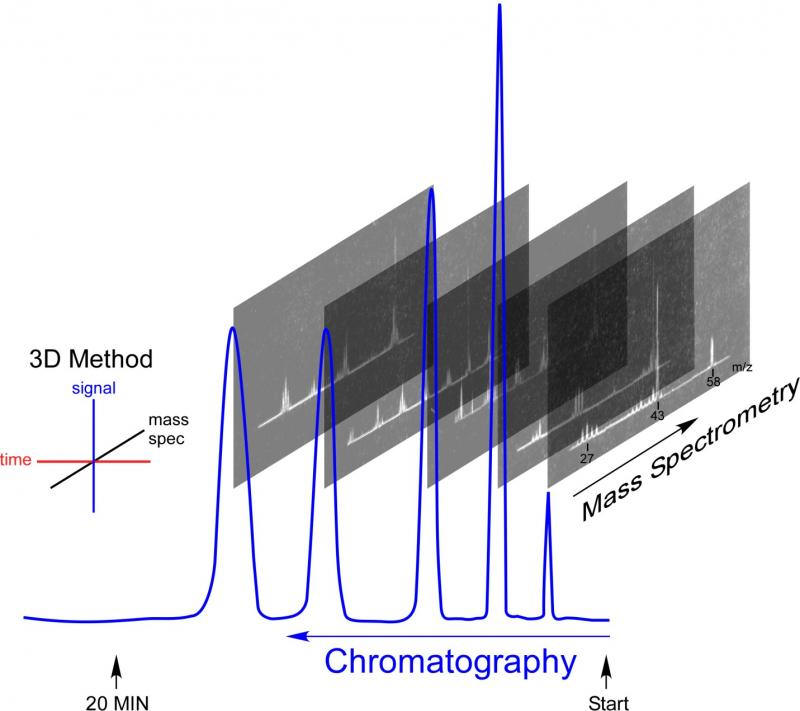
Delving into the history of the GC-MS recalls a time when both gas chromatography and mass spectrometry were in their infancy. It was a time of rapid innovation, with methods and equipment in flux. In GC-MS, chromatography separates a mixture into individual components, with each chromatographic peak being analyzed by a mass spectrometer. Components are identified unambiguously when both characteristic retention times and mass spectral fingerprints match reference materials. When analyzing unknown materials, the mass spectrum provides tentative identifications, dramatically reducing the number of possible matches. Because of its power and sensitivity, the technique is widely used in medicine, forensic analysis, environmental testing, drug testing and more. I used it in grad school to investigate ion-molecule reactions to confirm reaction mechanisms.  It was purely curiosity-driven research that leveraged the sensitivity of GC-MS for trace analysis.

GC operates by taking advantage of the differing affinities different vapors have for surfaces. A mixture is first vaporized by rapid heating is a flow of gas. The vapor and the carrier gas are pushed into a tube that in the 1950s was packed with small particles. Properties of the solid particles, like porosity or nature of a coating, slow some compounds more than others. In the race to get through the column, small, light compounds get to the end faster than big, heavy ones.  Watching at the end of the tube or column with a specialized detector produces a signal as each compound elutes or exits from the column. Plotting the signal gives a peak for each component in the mix.  Run in the same way, the pattern of peaks is reproducible. Compounds can be identified based on the time it takes to get through the column, the retention time. Calibrating a GC with known compounds gives the ability to identify components in a mixture based on retention time. Powerful as it is, chromatographic retention time alone is insufficient to unambiguously identify a component in a mixture. There is always a chance that two chemicals will have the same retention time. 

The GCs used in the first GC-MS were built by Roland Gohlke at Dow. Roland Gohlke packed his own GCs columns.  Tide detergent powder was a common packing.  It is said everyone knew when columns were being packed due to the distinctive detergent smell permeating the entire site. Columns were loaded in one of the taller stairwells and then coiled once filled. 

The instrument I encountered in grad school was designed for use with packed columns, though Tide detergent powder was no longer the packing of choice.  I could actually order columns from a catalog with a wide variety of packing options. 

Mass spectrometry was also in its infancy in the late 1950s. Most instruments still harkened back to J.J. Thomson’s earliest work with cathode ray tubes where bending ion beams with a magnetic field created patterns distinctive to the ionized substances.  All mass spectrometers work under vacuum.  Ions are manipulated and accelerated with electric fields, ultimately hitting a detector.  In 1955, mass spectrometers were being sold by a few manufacturers. These more-advanced instruments could identify analyze pure materials pretty well, and understanding of how molecules fragmented when hit by electrons led to the development of ways to use the spectra to determine molecular composition and structure.  For every chemical, a spectrometer produced a chart or “mass spectrum” that revealed the structure of the original, intact molecule. Any compound will break into the same ions under the same conditions, creating a unique mass spectrum, a fingerprint that can be used to identify the material.  70 V became the standard electron energy and libraries of mass spectral fingerprints soon became available to aid in the identification of unknown materials. When two or more materials are present, the mass spectrum is a combination of the spectra of each of the components. Rather than a clear fingerprint, the result is a mess that can’t always be used to identify and quantify the components. MS is great for pure materials, but not so great for mixtures. 

Mass spectrometers typically measure either a raw or amplified ion current, letting the ions directly create a measurable current. Magnetic sector instruments of the mid-1950s accelerated ions produced by shooting electrons through a vapor. Substances were leaked into an ion source and directed through a magnetic field where the collection of ions bends and separates like light through a prism. These magnetic sector instruments were cumbersome and slow.  Detroit-based Bendix Corporation introduced commercial time-of-flight instruments in the mid-1950s. These pulsed an ion source and accelerated the resulting ions through a long drift tube. The velocity of any ion, and, therefore, the time it took to traverse the drift tube, were dependent on the mass-to-charge ratio. Amplifying the current resulting from the ions hitting a detector at the end of the drift tube yields a full mass spectrum for each pulse of the ion source. Mass spectra could be read out directly on an oscilloscope rapidly, much more rapidly than a magnet could be scanned. 

When Fred McLafferty heard about the Bendix time-of-flight mass spectrometer, he knew that its speed could make it possible to couple with a GC. He reasoned that adding the power of mass spectrometry to identify pure components with the power of chromatography to separate a mixture into pure components would be more than additive. Adding a third dimension of data overcomes and compensates for the shortcomings of each individual method. Matching the retention time and mass spectra of a compound would seal the identification in a way chromatographic retention time alone could never do. Using chromatography to separate a mixture into pure components allows identification and quantitation impossible by taking a mass spectrum of a mixture. 

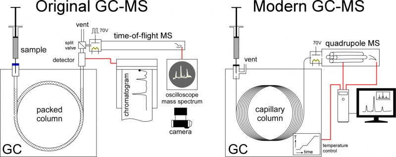
McLafferty and Gohlke faced an immediate problem, pressure.  GCs operate at pressure and mass specs operate under vacuum. Their solution was to use a leak valve they made, putting only part of the GC flow into the ion source.  A thermal conductivity detector recorded the chromatogram while spectra showed up only on an oscilloscope. This was far before computer data acquisition was possible and there was no way to record the electronic signals directly. A camera, manually triggered when a chart recorder showed a chromatographic peak was eluting, captured the mass spectra for analysis. The first paper McLafferty and Gohlke published shows photographs of the oscilloscope screen showing the mass spectra.  This gave way to an ultrafast chart recorder, the first of many modifications in the evolution of GC-MS to the devices of today. 

Mass spectrometers work on several different principles. The Bendix MS used by Gohlke and McLafferty was a time-of-flight (TOF) instrument where the time it took ions to traverse a long tube produced a spectrum. Bendix began marketing a GC-MS device in 1959, but the first commercial success was LKB Instruments Inc.’s Model 9000, which debuted in 1965. The LKB instrument was a magnetic sector instrument, now sped up enough to match the chromatogram.  Gone was the need for a separate GC detector, MS was now the detector. Other companies followed suit, including Finnigan Instruments, Perkin Elmer, and Hewlett Packard, now Agilent.  Several other advances paved the way for GC-MS to go mainstream.  The first was the development of small, fast mass filters that were far superior to the TOF or magnetic sector instruments.  The introduction of the quadrupole mass spectrometer made possible smaller, less expensive GC-MS. The GC-MS I first encountered was one of the first sold as a benchtop unit, though the computer required to run it effectively was a bench. 

The bench contained a computer that still required manual setting of switches on the front panel to get it to boot.  It had 16-inch disk platters that could hold a whopping megabyte of data.  While primitive by today’s standards, data acquisition and instrument control played a large part making GC-MS into the powerful tool it is today. Standardization of ionization energy meant that all MS units produce the same fingerprint for the same compound. Libraries of mass spectra were digitized so that computer matching was possible. GC-MS systems could now automatically identify chromatographic peaks. Computer control also allowed temperature control the GC. The ability to ramp temperature shortened elution times and narrowed chromatographic peaks, improving detection.

Improvements in vacuum technology were also important. Technology evolution occasionally results in extinction. The design of my old GC-MS is extinct. The idea of hanging a quadrupole in the throat of a diffusion pump, while novel and space saving, perished as pumps improved. Turbomolecular pumps replaced cumbersome and messy diffusion pumps. Production of oil-free vacuum systems reduced contamination and maintenance, dramatically improving operability of systems.

By the time I encountered my first GC-MS, the leak valve was gone replaced by several technologies able to better preserve the temporal resolution of the chromatogram. Mine, as received, used a membrane separator that rejected the helium carrier gas, while passing organic components. The promise of capillary or wall-coated open tubular (WCOT) chromatographic columns prompted me to jettison packed column chromatography.  This required several modifications but provided a big payout for trace analysis.  No more separator. Instead, the small flow out of the WCOT column would all go directly into the ion source. Samples would actually be split at injection port, letting only a little bit into the column. The superior resolving power of the capillary column gave narrower, easier to detect peaks. The widespread adoption of wall-coated, open tubular or capillary columns, replacing packed columns, is another important advance. These columns work well with very small amounts of material, well-suited for the great sensitivity of MS. They also provide very narrow, sharp chromatographic peaks, easier to for the MS to detect. Their improved resolving power makes GC-MS even more powerful for trace analysis.

The Invention of the GC-MS spawned a number of other hyphenated techniques. Coupling liquid chromatography with MS gives LC-MS.  GC with infrared spectroscopy gives GC-IR.  The list goes on, all started with the first coupled technique, GC-MS.

My hope of never seeing another GC-MS after graduate school didn’t work out. GC-MS was impossible to avoid during my career. The power of the technique made it the right choice for several projects. Simultaneous coupling of two columns into the MS so that permanent gases can be shunted by valving directly to the MS and concentrations determined by deconvolution is something I’ve used in process research that is only possible thanks to the power of GC-MS.  

Advances in both chromatography and mass filters continue with no sign of stopping.  Self-contained portable GC-MS units capable of being carried with one hand are now on the market.  These allow analysis on-site at crime scenes, environmental events, fires and more.  Bigger, more powerful GC-MS units still populate labs for particularly careful analyses.  GC-MS is now the go-to technology in modern chemistry labs. Applications include development of new pharmaceuticals and analysis of their purity, detection of chemical warfare agents and explosives, screening of athletes’ urine for banned performance-enhancing substances, and checking food quality and safety.  The technology has come a long way from the foundational experiments of Gohlke and McLafferty.  There pioneering work demonstrated that it was possible to couple GC with MS to create an exceedingly powerful tool.  They never could have grasped how powerful, how ubiquitous or how important the technique would become. 

edited to correct spelling errors for publication on mjphd.net on 19 July 2019